You might have read the first chapter of this series a few days ago, the idea was to see if that was something that people were willing to check before I invested too much time into writing this, but it seems people are eager to learn more about data science e see how that is applied to real businesses and real needs.
In this series, I’ll share how I tackled three different challenges and how I used data science to produce some great tools in the e-commerce project I was working back then, the challenges were:
- How can I predict how much money we will make next month?
- What customers clusters we have and what defines them?
- Can I predict a customer quality as it puts its first order?
In this chapter, I’ll talk about the first point, how I was able to predict the e-commerce monthly revenue with a margin of error of 10%.
Tools
For this initial challenge I used numpy, pandas and sklearn, we will also use two different Machine Learning algorithms, the classic Linear Regression and one way more complex called Gradient Boosting Regressor, worry not, I’ll explain how each one works so bear with me.
I’ll start by importing everything I need:
# Importing necessary libraries
import pandas as pd
import numpy as np
import seaborn as sns
import matplotlib.pyplot as plt
from sklearn.linear_model import LinearRegression
from sklearn.ensemble import GradientBoostingRegressor
%matplotlib inline
plt.style.use('fivethirtyeight')
plt.rcParams['font.serif'] = 'Ubuntu'
plt.rcParams['font.monospace'] = 'Ubuntu Mono'
plt.rcParams['axes.labelweight'] = 'bold'
plt.rcParams['xtick.labelsize'] = 15
plt.rcParams['ytick.labelsize'] = 15
Assesment
Starting from an empty Jupyter notebook I poked a bit around the orders data I had.
# =======================================================
# Read Orders data by day
# =======================================================
orders = pd.read_csv('orders.csv')
# Convert datetimes to pandas datetime type
orders["created_at"] = pd.to_datetime(orders.created_at)
orders["processed_at"] = pd.to_datetime(orders.processed_at)
The main goal of this part was to gain some domain knowledge, understand what were the main factors that drive the revenue for a specific month, those are the factors that we want to feed into the prediction mode.
The first thing that I noticed when plotting the orders by month was that there was some seasonality and that the month of the year has a huge influence on the revenue as you can see below:
# Getting paid Orders only.
# ============================================================
orders = orders[(orders.paid == True) & (orders.canceled == False)]
by_month_data = orders.month.value_counts().sort_index()
f, (ax1) = plt.subplots(1, 1, figsize=(25, 10))
plot = sns.barplot(by_month_data.index, by_month_data.values, ax=ax1)
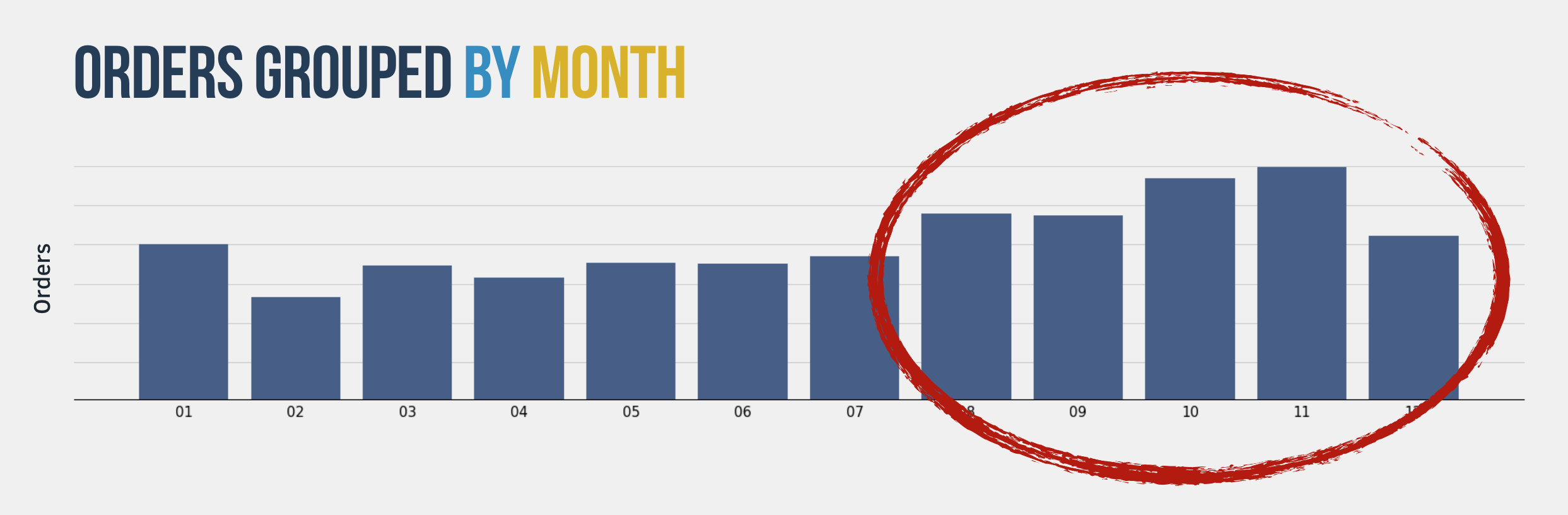
So the month of the year is definitely a data that we need to feed into our prediction model.
I had only 3 years worth of data, but that was enough to check how much a month revenue correlates with all other months revenues:
from statsmodels.graphics.tsaplots import plot_acf
f, (ax1) = plt.subplots(1, 1, figsize=(25, 8))
plot_acf(monthly_data.revenue, ax=ax1)
pyplot.show()
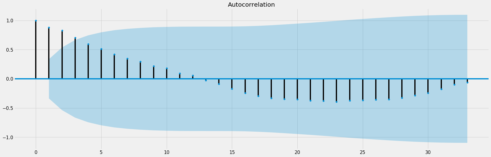
Each point on this graph indicates how much one month correlates with the other months, axis X representing all months I have, 33 months, and axis Y representing the correlation index, here we can see that a specific month has a high correlation with the point 12 and 13, that indicates that a month’s revenue is highly correlated to the same month’s revenue one year before.
Basically what it means is that if you had a good revenue in January last year that might imply on a good January this year, the monthly revenue tend to follow a pattern. This means that the revenue from the same month but on the last year is another data that we need to feed into our Machine Learning model.
More Data
Now that I had some insight into the data I had it was time to put together other data that might have a say in predicting in predicting the revenue for a month.
After some poking around I found other data that was worth having: The Ads Investment ($) it was planning on doing that month.
Once I had all the data in hand was the time to apply to Machine Learning on it, the data I decided to use was:
- Last year’s same month revenue
- Last month’s revenue
- $ spent on Ads for the current month
- What month it is
- What season it is
Trying Linear Regression
Known as one of the simplest ML algorithms, linear regression is pretty straightforward and rely on you having data that have a linear relationship.
I spare the last 4 months of my data so that I could test my prediction model and see if it would have guessed how much the revenue would be for those.
test_data = final_data[-4:]
final_data = final_data.drop(test_data.index)
X = final_data[feature_cols]
y = final_data.revenue
linreg = LinearRegression()
linreg.fit(X, y);
f, (ax1) = plt.subplots(1, 1, figsize=(20, 8))
X = test_data[feature_cols]
y = test_data.revenue
ndf = pd.DataFrame(y)
values = linreg.predict(X)
ndf['estimates'] = values
ndf['difference'] = ndf.estimates - ndf.revenue
ndf
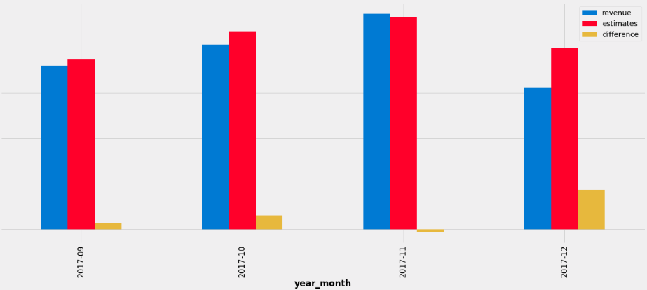
plot = ndf.plot(kind='bar', ax=ax1);
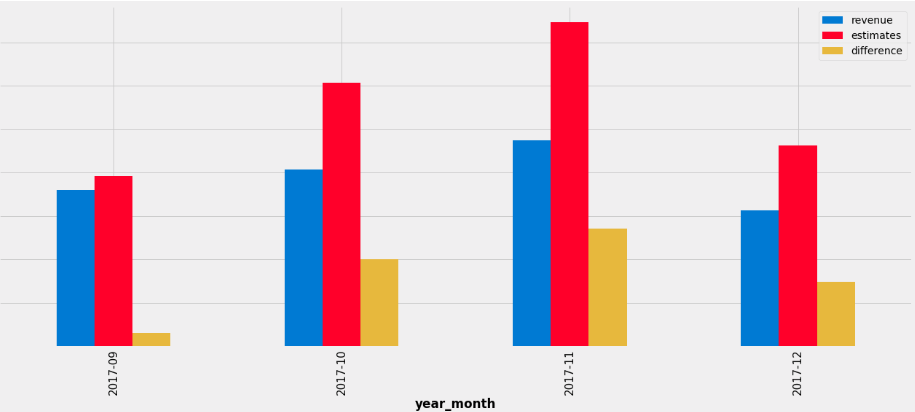
The prediction was okay, but it wasn’t as effective as I wanted it to be, in some months, like November it missed by more than 30%, and that wasn’t as helpful as I needed it to be taking into account we wanted to use this intel to better prepare ourselves, to be more proactive than reactive in terms of the business in general.
So I decided I needed a better ML (Machine Learning) model that could better capture the relationships between the data that I had.
Trying Gradient Boosting Regressor
I decided I needed a model that could capture more complex relationships other than linear, and while looking for it I learned about the Gradient Boosting Regressor, it seemed awesome, but the issue is that it’s based on Decision Trees, and Decision Trees are good on predicting values that it already knows, but there is no way it could predict a value it has not yet seen, and that was exactly the case because we as an e-commerce startup were going through a huge growth so our numbers kept growing as well, and it would be impossible for the algorithm to predict a revenue higher than the ones it has already seen.
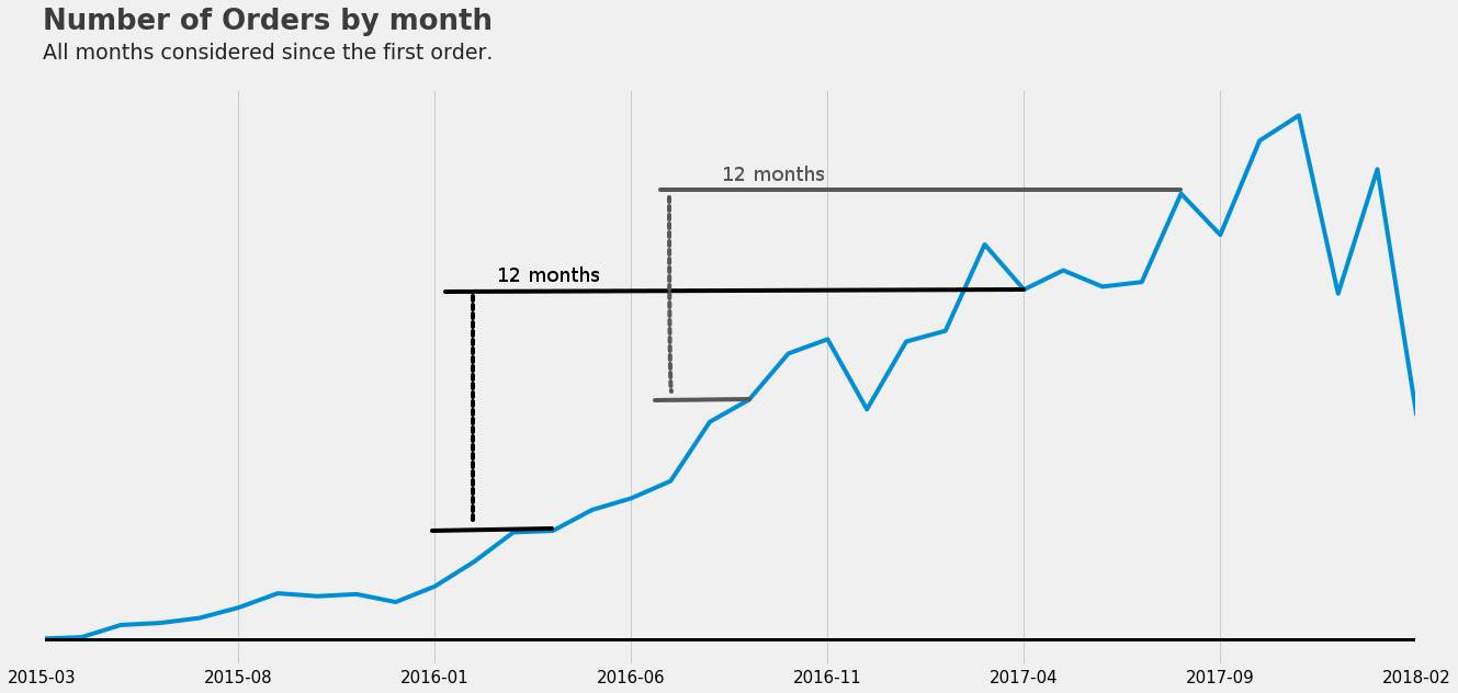
So that is when I learned about how to deal with trends and use a method called Random Walk. First, let’s check the trend over the past years of data:
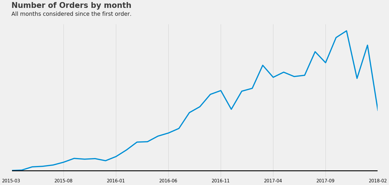
P.S. the drop on the end of the chart is because it was missing the how of the last month worth of data.
This chart shows a trend in the number of orders, the same trend occurs on the revenue and the fact that we are always increasing the revenue is what makes it hard for us to use a Decision-Tree-based model, but what if instead of estimating the revenue we could estimate another value that is kept under a range? You got it, instead of estimating the revenue we can estimate the difference between the current monthly revenue and the same month’s revenue from the year before.
As you can see the difference is kept under a usual range, sometimes more and some less but within a range and that enables us to use a Decision-Tree-based model, so all we have to do is to estimate the difference and then sum it up with the revenue from the same month one year before.
Once I’ve trained the model this is the results I got for the same 4 last months of the year:
P.S. there was some tunning to figure out the best number of trees and the maximum depth of each tree.
f, (ax1) = plt.subplots(1, 1, figsize=(20, 8))
X = final_data[feature_cols]
y = final_data.revenue - final_data.last_year_same_month_revenue
X_test = test_data[feature_cols]
ndf = pd.DataFrame(test_data.revenue)
params = {'n_estimators': 1540, 'max_depth': 2}
est = GradientBoostingRegressor(**params).fit(X, y);
ndf['estimates'] = est.predict(X_test) + test_data.last_year_same_month_revenue
ndf['difference'] = ndf.estimates - ndf.revenue
plot = ndf.plot(kind='bar', ax=ax1)
Here is a comparative on how it predicts better when compared to a just simple linear regression, check how close the GradientBoostRegressor algorithm + Random Walk got when compared with the Linear regression.
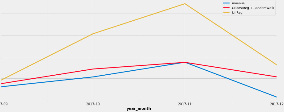
As you can see the new algorithm performed way better and is still live in production producing results within a margin of error of 10%.
Once I had the prediction model it was only a matter of exporting it and making it an API so that I could integrate it with an dashboard.
This way the business can now predict the next month revenue and properly prepare for it.
Next Steps
I hope you have liked this article I tried to not make it too technical while also sharing some code so you can try out some cool stuff on your side as well, I’m not sure if I will be able to share all the code involved because of confidentiality concerns but I’ll make sure to share as much as I can.
If you liked this chapter make sure to let me know on Twitter, it makes a huge difference getting me pumped and willing to write more about it.
On the next chapter, I’ll talk about the second challenge: What customers clusters we have and what defines them?